In my last post I briefly introduce how I set up Apache Spark on my own laptop. In this post, I will start using Spark and Python to do some data exploration.
Resilient Distributed Datasets
Let’s first get familiar with how Spark store data. The Resilient Distributed Datasets (RDD) is the core concept of Spark. An RDD is a collection of “records” that is distributed or partitioned across many nodes in a cluster.
The RDD is fault-tolerant, which means if a given node or task fails, it can be reconstructed automatically on the remaining nodes and the job will still complete.
Data
The dataset I will use is called MovieLens 100k (it can be downloaded here). It contains 100,000 data points related to ratings given by a set of users to a set of movies. It also contains movie metadata and user profiles. It is applicable to recommender systems as well as potentially other machine learning tasks. Therefore it serves as a useful example.
Examples of other publicly accessible datasets include
Exploring the user data
%matplotlib inline
import seaborn as sns
import pandas as pd
user = sc.textFile("E:/Documents/zhoujli.github.io/_source/ml-100k/u.user")Let’s first take a look at the user information. The take(k) function collects the first k elements of the RDD to the driver. If you are familiar with pandas, it is very similar to the head function.
user.take(5)[u'1|24|M|technician|85711',
u'2|53|F|other|94043',
u'3|23|M|writer|32067',
u'4|24|M|technician|43537',
u'5|33|F|other|15213']
We can see that each line of the data is a combination of several fields of user information (user ID, age, gender, occupation and ZIP codes), separated by the “|” character. The next step is to split them. The map operator applies a self-defined function to each record of an RDD, thus mapping the input to some new output. In Python, it is easy to define a function using lambda.
user_fields = user.map(lambda line: line.split("|"))
user_fields.first()
[u'1', u'24', u'M', u'technician', u'85711']
After the fields are seperated, we can start playing around with the data. We may ask questions like below.
- How many unique users?
- How many unique genders?
- How many unique jobs?
- How many unique ZIP codes?
It is easy to answer the above questions using the distinct and count functions.
num_users = user_fields.map(lambda fields: fields[0]).distinct().count()
num_genders = user_fields.map(lambda fields: fields[2]).distinct().count()
num_occupations = user_fields.map(lambda fields: fields[3]).distinct().count()
num_zipcodes = user_fields.map(lambda fields: fields[4]).distinct().count()

print "Users: %d, genders: %d, occupations: %d, ZIP codes: %d" % (num_users, num_genders, num_occupations, num_zipcodes)
Users: 943, genders: 2, occupations: 21, ZIP codes: 795
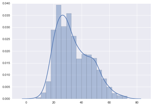
We can also visualize the distribution of user ages. Here I am using the distplot function provided by Seaborn.
As we can see, the age distribution is right-skewed (with long tail on the right). A large number of users are around 15~35.
ages = user_fields.map(lambda x: int(x[1])).collect()

sns.distplot(ages)
<matplotlib.axes._subplots.AxesSubplot at 0x8659630>
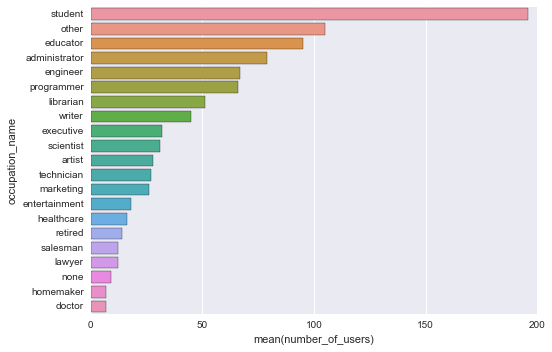
What if we want to know number of users by their occupations?
We can first map each user’s occupation to a (key, value) pair, where key is occupation and value is 1. For example, (‘student’, 1).
Then, the reduceByKey function will merge the values for each key using an associative reduce function. This will also perform the merging locally on each mapper before sending results to a reducer, similarly to a “combiner” in MapReduce.
Finally, we collect the output and save it in a pandas DataFrame, sort by count, and plot it.
count_by_occupation = user_fields.map(lambda fields: (fields[3], 1)).reduceByKey(lambda x, y: x + y).collect()
c_by_o = pd.DataFrame(count_by_occupation, columns=['occupation_name', 'number_of_users']).sort_values('number_of_users', ascending=False)
sns.barplot(x='number_of_users', y='occupation_name', data=c_by_o)
<matplotlib.axes._subplots.AxesSubplot at 0xbf0f9e8>